Use case: Drift detection on the edge using the disentangled latent space of an autoencoder (LSDD)

Introduction

In industry, the production environments where machine learning (ML) models are deployed often look different from the R&D environments in which the models are trained. These environments are also dynamic, changing over time because of factors like other machines, weather and malfunctions. These changes can cause the ML model to degrade over time which is why ML models often stay in the R&D phase and never get deployed into the production environment. To solve this problem, drift detectors were created to detect when the environments change in such a way that the model starts performing worse. There are two main types of drift detectors. The first type are supervised drift detectors, which use the true labels of a model to calculate its accuracy or error rate to detect drift. When these metrics worsen, there is a drift happening. These detectors assume that there are always immediate true labels available but this is often not possible in production. Therefore there is a second group of drift detectors, the unsupervised drift detectors, which use other techniques to detect drift in the input data of the ML model to predict when the ML model might be degrading in performance.

At the same time, the field of edge ML is starting to rise. Normally ML models are trained and deployed on the cloud. However, when working in a production environment, using a model deployed on the cloud could cause problems. For example, constantly sending data to the cloud and back can cause a lot of latency in the results of the ML model. Second, it requires a lot of bandwidth to constantly send and receive data. This could be fine for a single machine but could cause problems if the same ML model is needed for several machines. Next, when data is sent to the cloud it could get intercepted, which can cause privacy problems. Lastly, in some situations there is no connection to the cloud available. In those cases it might be best to deploy the ML model on edge devices, close to or on the machines themselves. However, ML models can be very computationally expensive, and running these models on an edge device will require consideration of the ML model's size.

If the ML model is running on the edge, the drift detection process should also be close to the edge to detect drift as fast as possible. However, this process needs resources which are not available on a small edge device, like saving inputs or training an ML model. Therefore, a novel drift detection technique is introduced which detects drift in a resource-efficient way through the use of the latent space of an autoencoder. In this use case, we evaluated this new drift detector on two demonstrators. These are the Beckhoff motor bearing setup and the CTRL-Engineering magic marble machine.

Method

The introduced technique is called the Latent-space drift detector (LSDD). It uses the latent space of an autoencoder to detect drift in the data. An autoencoder is an ML model consisting of two parts. The first part is the encoder which creates a smaller embedded version from the input data. The space that the embedding vector creates is called the latent space. The second part of the autoencoder is the decoder which reconstructs the input data from the embedded representation. To be able to detect drift, the latent space of the autoencoder needs to be disentangled. This means that the different dimensions of the latent space each have their own interpretation of the input data independent from the other dimensions. Ideally these interpretations are understandable to humans. This disentanglement is created through the use of an orthogonal autoencoder (OAE), which forces orthogonality on the latent space vector. The LSDD consists of three stages which are explained in the next subsections.

The offline training stage

The first step of the LSDD technique is to create an orthogonal autoencoder on the training data. To create the most optimally disentangled latent space, the OAE is optimized through the use of hyperparameter optimization. The used optimization metric is the silhouette score which shows how well a certain set of data is clustered. In this case the clustering of the training data based on their classes in the latent space should have the best silhouette score. Once a good disentangled latent space has been found, the decoder part is removed and a new hyperparameter optimization is initiated which finds the optimal task layers for classifying the training data. After this, the different class means and variances of the training data in the latent space are calculated after which LSDD is ready to start the online drift detection process.

The online drift detection stage

The online drift detection stage is where the detector is deployed on the edge device and starts evaluating the input data. At every input sample the distance between the new data sample to the current class mean in the latent space is calculated. Depending on the results, drift is detected and the task layers should be adapted

The offline model adaptation stage

When drift is detected, the task layers are adapted. There are two main ways in which this could be done. First, a new concept can be detected, which means new data is collected and the task layers are retrained. However, once a concept is known it can be reused when it returns, without retraining, which is the second way the layers could be adapted.

There are several hyperparameters to set with this drift detector, which set the sensitivity of LSDD. The same is true for other drift detectors, like D3, which is used to compare the LSDD algorithm. Therefore, a multi-objective hyperparameter optimization is used which tries to optimize the results of the drift detection based on three metrics. These metrics are the mean time to detection, the mean detection ratio and the number of false detections. All these metrics should be as low as possible. This optimization gives us some optimal hyperparameters for the given datasets and methods. In addition to these results, the memory usage and algorithm speed of the two drift detectors is measured.

The setups

The new drift detection technique is evaluated on datasets from two demonstrators. These are the motor bearing setup from Beckhoff and the magic marble machine from CTRL-Engineering.

Motor bearing setup

This setup contains a motor with four different types of bearing. The original ML model is trained to detect the different types of bearings based on the vibration sensor data. The training dataset only contains data where the motor speed was 30 rev/s. However, the motor can also rotate at slower speeds, which change the data and reduces the model accuracy. The different motor speeds represent the different concepts that LSDD needs to detect. The collected dataset contains three drift points, switching between 10 and 30 rev/s.

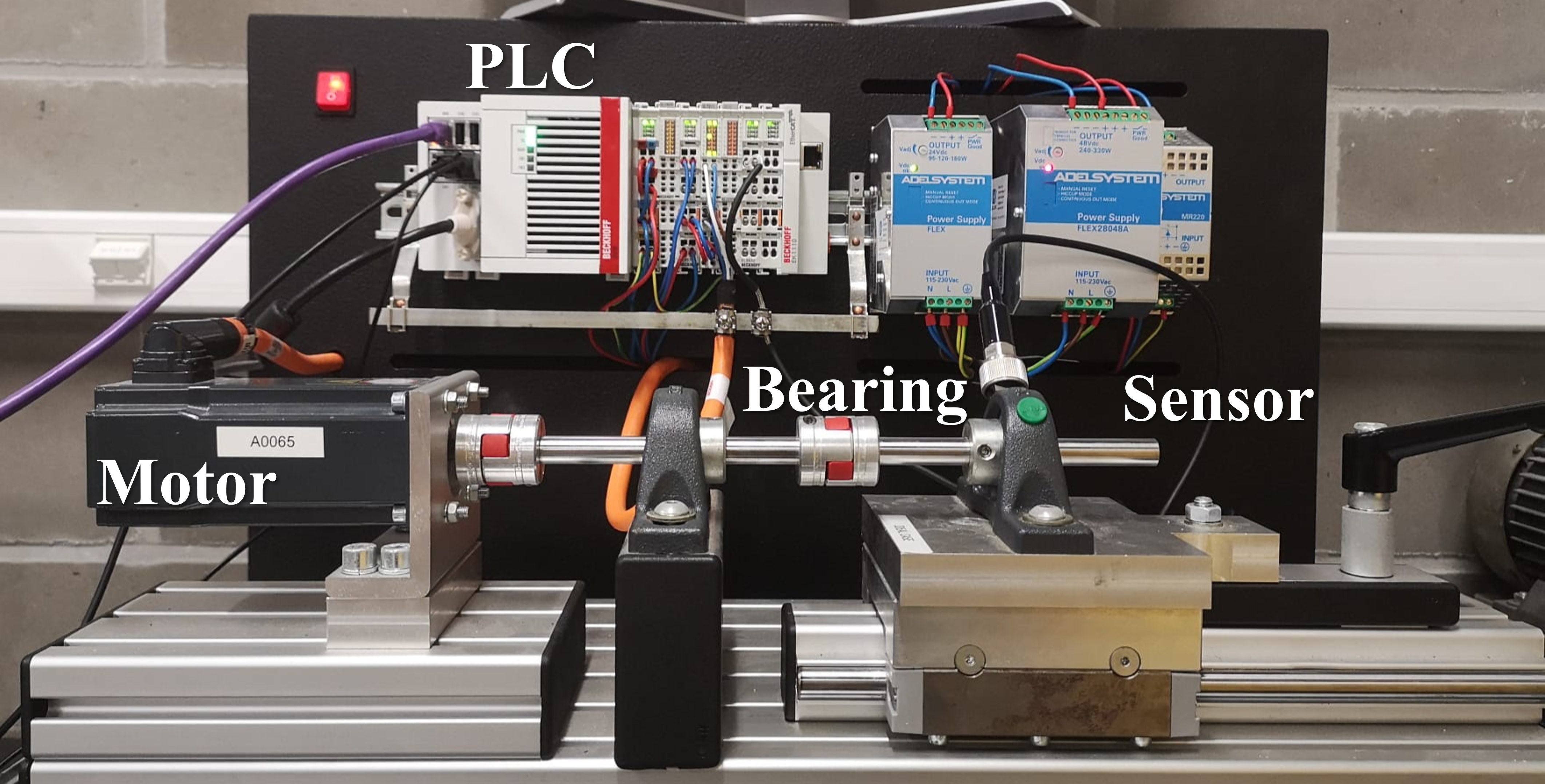
Figure 1: The full motor bearing setup containing an ideal bearing.

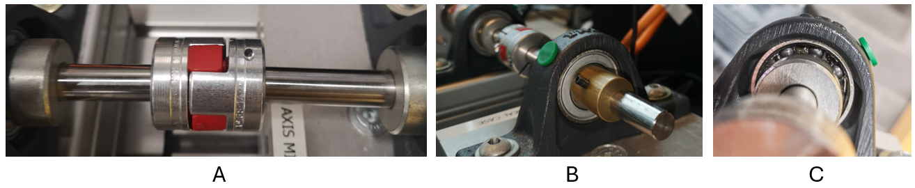
Figure 2: The different types of faults in the bearing: A) axis misalignment. B) imbalanced weight. C) faulty bearing.

Magic marble machine

This second demonstrator contains an ML model which can sort marbles based on colors. However, the marble dataset contains pictures of marbles in a certain lighting setup. When this lighting setup changes, it has an effect on how well the model is able to sort the different colored marbles. Therefore, we want to detect drift when the lighting setup changes and the model might be degrading. We create two different lighting setups by artificially changing the brightness of the collected marble dataset. This gives us two different concepts: bright and dark. The original ML model task is to classify the different images based on the colors of the marbles. This gives us four classes: black, white, blue, and empty (when there is no marble in the image). Using this adapted data, we create a streaming dataset which changes concepts nine times, switching between the bright and dark images, which will be used to evaluate the drift detectors.

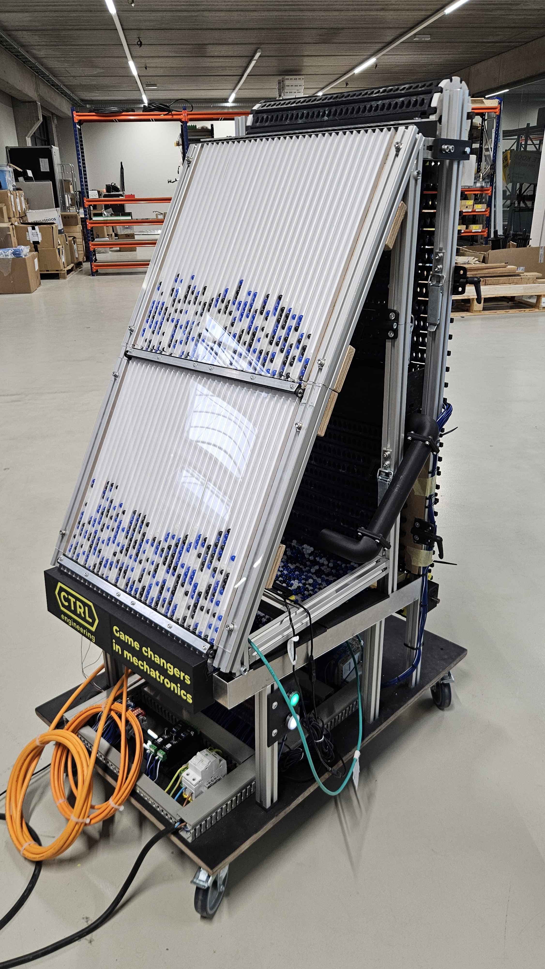
Figure 3: The magic marble machine.

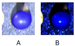
Figure 4: The two different concepts for the magic marble machine: A) the bright images. B) the dark images.

The experiments and results

LSDD is compared to D3, a well-performing drift detection technique, on the two datasets on two different aspects. The first aspect is the accuracy of the drift detection measured by three metrics: mean time to detection, mean detection ratio and number of false detections. The second aspect is the resource usage of the drift detection techniques. To measure this, both the memory usage and the processing power, represented by the execution time, are used. LSDD and D3 have hyperparameters which set the sensitivity of the drift detector. To make sure these parameters are optimized for the dataset, a hyperparameter search is implemented for both techniques and the best performing results are compared to each other. The results, which can be seen in the tables and figures below, show that LSDD performs as well as D3 in detecting the drifts and does so with less memory and processing power.

Table 1: Drift detection results of LSDD and D3 methods on the magic marble dataset.

Algorithm	Parameters	MTD
LSDD	N=65, γ=0.07, K=84	306.44
D3	w=125, ρ=0.109, threshold=0.868, K=94	315.77
D3	w=105, ρ=0.101, threshold=0.911, K=83	315.77

Table 2: Drift detection results of LSDD and D3 methods on the motor bearing dataset.

Algorithm	Parameters	MTD	MDR
LSDD	N=13, γ=0.077, K=73	2.666	0
LSDD	N=10, γ=0.050, K=74	2.666	0
D3	w=82, ρ=0.544, threshold=0.6525, K=47	8.5	0.333

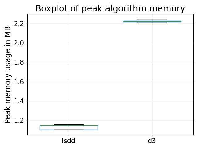
Figure 5: The peak algorithm memories for both LSDD and D3 showing a better performance for LSDD on the magic marble dataset.

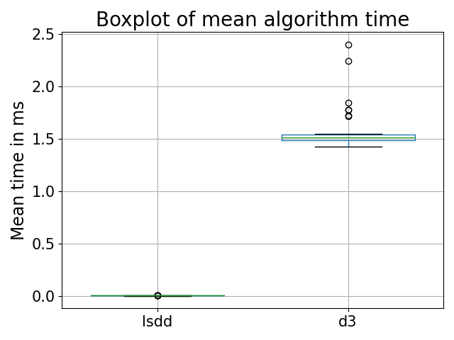
Figure 6: The mean algorithm times for both LSDD and D3 showing a better performance for LSDD on the magic marble dataset.

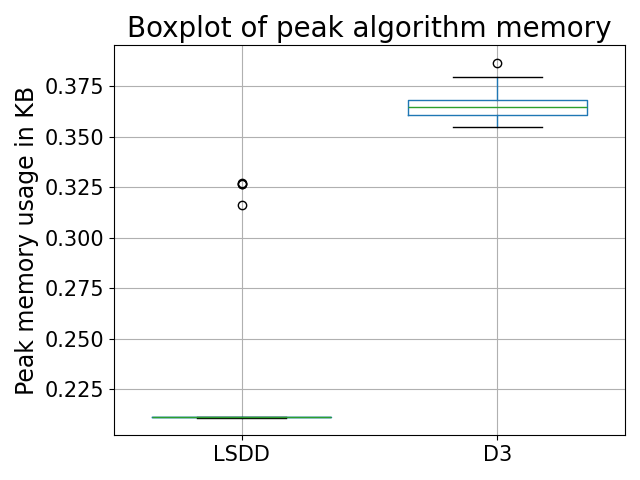
Figure 7: The peak algorithm memories for both LSDD and D3 showing a better performance for LSDD on the motor bearing dataset.

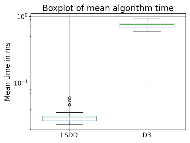
Figure 8: The mean algorithm times for both LSDD and D3 showing a better performance for LSDD on the motor bearing dataset.

Conclusion

This use case uses a new drift detector called LSDD which uses the latent space of an orthogonal autoencoder to detect drift in an unsupervised, resource efficient way. Compared to D3, a well-performing drift detection technique, LSDD performs better on two datasets in both drift detection accuracy and resource efficiency. If you want to learn more about LSDD, it will be published in a workshop paper for the MLOps workshop of ECAI which will be made available on this page after publication.